Every latency number answers one question
The dashboard was right; it was timing a different wait.
On this page · 9 sections
- Four questions, four useful numbers
- The mean earns its place in capacity planning
- A p99 leaves one request in a hundred beyond it
- Checkout waits for the slowest call
- An averaged p99 can be wrong in either direction
- Add counts, then divide
- The wait your load test never timed
- What I’d put on the dashboard
- Run the model, then the measurement experiment
The pricing service’s dashboard looks healthy: a mean of 23.4 ms, and a p99 of 49.0 ms, which means 99 requests in 100 finish in 49.0 ms or less. A customer writes in to say that checkout keeps hanging.
Both are true. Checkout asks the pricing service for the price of each item in the basket, 20 calls at once, and waits for every answer. The service measures one request at a time. The customer waits for the slowest request in a group of 20.
Behind the service’s load balancer are four hosts. Three behave normally. The fourth, host 4, has a garbage-collection pause, a moment where the process stops to tidy its memory, that catches 2% of its requests and adds 300 to 600 ms to each. With traffic shared roughly equally, that affects about half a percent of all requests. That is too few to move the service’s p99, and it’s enough to slow 9.1% of checkout pages.
This service is a model I wrote for this post, not a production incident. It draws 100,000 requests from a seeded generator, so the companion code reproduces every number below exactly. The load-test experiment near the end uses a real TCP server, so its timings vary by machine.
The short version
- The mean (23.4 ms) tells you how much capacity you need. It doesn’t tell you how long any one customer waits.
- The p99 (49.0 ms) hides whatever happens to fewer than 1 request in 100. Host 4’s stalls hit about 1 request in 200, so the p99 never sees them.
- A page that waits for 20 calls is as slow as the slowest. About 1 slow request in 200 becomes 9.1% slow pages.
- Averaging the four hosts’ p99s gave 149.5 ms against a true 49.0 ms, three times too high. Put most of the traffic on host 4 and the same average comes out at less than half the truth.
- The share of requests under 100 ms adds up exactly across hosts: 99,517 of 100,000, however you split them. That’s the promise to watch.
- A load test that waits for each reply before sending the next can miss most of a server’s freeze. Ours recorded 10 slow requests where users would have felt 392.
Four questions, four useful numbers
A pizza kitchen makes the distinction easier to see. The manager wants enough ovens and cooks for the orders in progress. A customer wants to know when their pizza will arrive. A table ordering five dishes waits for the last dish. Head office wants to know how often the chain kept its “30 minutes or it’s free” promise. To check that, each branch sends in two counts, orders and orders under 30 minutes, and head office adds them up.
Those are different questions about the same kitchen. A dashboard that answers one of them well may tell you very little about another.
| Who asks | The question | The number | How it rolls up |
|---|---|---|---|
| The manager | How much work is in flight? | The mean, times the arrival rate | Weight each host’s mean by its request count |
| One customer | How long does one request take? | A percentile of request latency, p50 or p99 | Pool the measurements, then compute |
| The table of five | How long does the whole page take? | The page’s own percentile, or the share of slow pages | Measure pages; a call’s percentile is not a page’s |
| Head office | How often did we keep the promise? | The share under a threshold | Add the counts under it and the totals, then divide |
The last column matters because almost every dashboard combines something, such as instances into a service, minutes into an hour, or regions into a global view. The rest of the post takes the four rows one at a time.
The mean earns its place in capacity planning
Means get blamed for hiding slow requests, and they do hide them. So the tail needs another number. The mean still does one job that no other number does.
Little’s law says that in a system that is stable over a window, the average number of requests in flight equals the arrival rate times the average time each one spends inside (Little’s law, proved by John Little in 1961). It holds whatever shape the latency distribution has, which is what makes it useful. At an illustrative 2,000 requests a second:
Little's law: 2000 req/s x 23.4 ms = 46.8 requests in flight on averageSo about 47 requests are inside the service at any moment, on average. That’s the manager’s question, and it is the starting input for sizing thread pools, connection pools and the number of hosts. Bursts and headroom still matter on top of it. A p99 can’t stand in for it, because a p99 describes one position in the list and says nothing about the total time all the requests spend inside.
What the mean can’t do is describe a request. Look at the hosts, in milliseconds:
== 100,000 requests, 25% of them on host 4, which stalls 2% of its requests by 300 to 600 mshost 1: 24,896 requests mean 21.3 p50 20.1 p99 44.9 under 100 ms 100.000%host 2: 25,196 requests mean 21.3 p50 20.0 p99 45.0 under 100 ms 100.000%host 3: 24,954 requests mean 21.3 p50 20.0 p99 45.3 under 100 ms 100.000%host 4: 24,954 requests mean 29.9 p50 20.1 p99 462.6 under 100 ms 98.064%...Host 4’s mean is 29.9 ms, and hardly any request on host 4 takes anything like 29.9 ms. Almost all of them take around 20 ms, and 2% take 300 to 600 ms more than that. The mean sits between two groups that don’t overlap, and it describes neither. Host 4’s median, its p50, barely moves, while its p99 lands squarely in the stalls.
The mean does add up across hosts, which is the other reason to keep it. But only if each host’s mean is weighted by its number of requests. With traffic spread evenly, that makes no visible difference. Put 70% of the traffic on host 4 and it does:
...means, weighted by requests: 27.6 ms = pooled mean 27.6 ms; unweighted average of means 23.5 ms...A dashboard that averages per-host means without weights reports 23.5 ms for a service whose real mean is 27.6 ms. That gives the quiet hosts the same say as the busy one, and it understates the mean by about 15%. Feed it into Little’s law and the requests in flight are undercounted by the same 15%. The fix is to add up the total time and the request count, then divide.
A p99 leaves one request in a hundred beyond it
A percentile is a position in the sorted list of measurements. The p50, the median, splits them in half. The p99 is the latency that 99% of requests come in at or under. The demo uses nearest rank: sort the values and take the one at position , rounded up.
def percentile(values: list[float], p: float) -> float: """Nearest rank: the smallest measurement with at least p% of the measurements at or below it.""" s = sorted(values) return s[max(0, math.ceil(p / 100 * len(s)) - 1)]It always returns a measurement that really happened, which is why I like it for latency. A p99 of 49.0 ms is a request that took 49.0 ms. It isn’t the only definition tools use, though.
Why two tools can report different percentiles
numpy and R default to linear interpolation. If the position falls between two measurements, they take a point between them. On 100,000 requests the two agree to a fraction of a millisecond. On 20 requests, or on a distribution with a gap in it like host 4’s, they can be far apart, because the position lands between a 45 ms request and a 400 ms one. Comparing a p99 from a tool that interpolates with one from a tool that doesn’t is comparing two different numbers, so check which definition each tool uses before comparing. The Percentiles across hosts tool further down shows both side by side for any raw latencies you paste.
For all 100,000 requests together, the model reports:
mean 23.4 ms, p50 20.0, p99 49.0, p99.9 552.7The p99 is 49.0 ms. The p99.9 is 552.7 ms. Between them sit host 4’s pauses, and it’s easy to see why they slip through. Host 4 takes a quarter of the traffic and stalls 2% of it, so stalled requests are about 0.5% of everything. A p99 only sees what happens to more than 1% of requests, so it can’t see this half a percent.
What the p99 does say is that 99 in 100 individual requests are fast. Checkout needs 20 of them.
Checkout waits for the slowest call
Leave rendering and other page work aside for a moment. All 20 pricing calls start together, and checkout can’t show the basket until every one is back. So the page’s pricing wait is the maximum of 20 request latencies, and a maximum finds the tail.
Say a share of requests is slow. For independent calls, the chance that none of them is slow is , so the share of pages with at least one slow call is . In the model, 483 of the 100,000 requests take 100 ms or more, so is 0.483%. The demo checks the formula against 20,000 simulated pages of each size:
== a page waits for its slowest call (20,000 pages each) 1 call : page p50 20.0 ms, page p99 48.8, pages over 100 ms 0.5% (1 - (1 - q)^N predicts 0.5%) 5 calls: page p50 29.9 ms, page p99 487.3, pages over 100 ms 2.5% (1 - (1 - q)^N predicts 2.4%)20 calls: page p50 38.8 ms, page p99 581.5, pages over 100 ms 9.1% (1 - (1 - q)^N predicts 9.2%)50 calls: page p50 45.8 ms, page p99 605.5, pages over 100 ms 21.5% (1 - (1 - q)^N predicts 21.5%)...At 20 calls, 9.1% of checkout pages take over 100 ms, from a service where 99.5% of requests are under it. The page’s p99 is 581.5 ms, while the service’s p99 is 49.0 ms. That’s the customer’s complaint, in numbers. Checkout is the table of five with 20 dishes. The order is as late as its slowest dish, and with 20 dishes one of them is slow far more often than any single dish is.
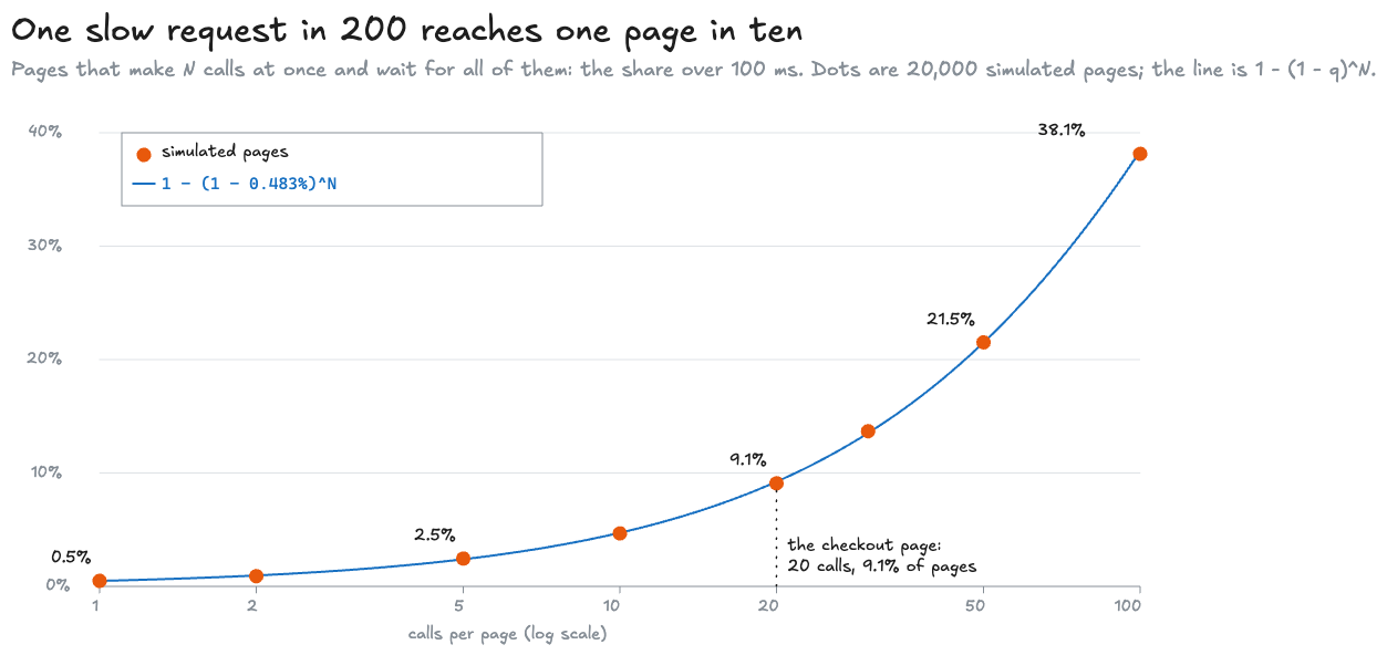
The same relationship translates percentiles. A page is faster than some time only if all of its calls are, so .
For the page’s -th percentile, set the left side to and solve: . So a page’s -th percentile is a request’s -th percentile. A percentile can have decimals: p99.95 is the latency that 99.95% of requests beat.
...20 calls: a page's median is a request's p96.6, and a page's p99 is a request's p99.95...Half of all checkout pages wait for a request slower than the service’s own p96.6. And to keep 99% of pages under 100 ms, every call’s p99.95 has to be under 100 ms. The call’s p99 isn’t strict enough. That’s the number the pricing team should be held to, and it’s one their dashboard doesn’t show. Dean and Barroso made this point famous in The Tail at Scale (2013), for servers that are slow one time in a hundred: “If a user request must collect responses from 100 such servers in parallel, then 63% of user requests will take more than one second.”
I end up doing this sum in a lot of design reviews, so I made it a tool. Give it how many calls one request waits for, the share of those calls that are slow (or the percentile that sits at your limit, so p99 means 1%), and the percentile you promise for the whole request. It answers both questions at once: the share of requests that wait for a slow call, , and the percentile each call needs for your target to hold. It opens on checkout’s pricing calls, 20 at 0.5% slow: 9.54% of requests, and each call needs its p99.95. The model’s own share, 0.483%, gives 9.2% by the formula and 9.1% simulated.
Most services don’t call one thing 20 times, though. They call a dozen different things, each with its own tail. For that, list the dependencies instead, one per line, such as pricing 20 0.5%. The tool multiplies each one’s chance of being fast, so the slow share is , and ranks them by what that share would drop to without each one. Press Checkout, 12 dependencies to see why that ranking matters: 34 calls a request leave 16.1% of checkouts slow, about one in six. Fixing pricing takes that to 7.26%. Fixing shipping quotes, the dependency with the worst p99, only gets it to 14.4%, because a request calls pricing 20 times and shipping once. And for a p99 checkout, each of those 34 calls needs its p99.97.
Where independence stops being a good assumption
The formula treats the 20 calls as independent. Real calls often aren’t. If host 4 pauses, every call routed to host 4 during the pause is slow together. That bunches slow calls into fewer pages, so fewer pages are slow than the formula says, but the ones that are slow are hit by several stalls at once. Other kinds of dependence can push the other way. So measure the page itself, and use the formula as the baseline to compare it with. The model draws each call independently, which is why it matches the formula so closely.
Different backends need different probabilities, too. If a page calls several backends, multiply each one’s chance of meeting the threshold, rather than raising one shared chance to a power. And a page that can render before every answer arrives has a different rule again.
The Tail at Scale’s remedies work on exactly this. A hedged request is a second copy of a call that’s running late, sent to another server, taking whichever reply comes back first. In the paper’s own benchmark, sending that hedge after 10 ms cut the p99.9 from 1,800 ms to 74 ms “while sending just 2% more requests.”
An averaged p99 can be wrong in either direction
Now the dashboard problem. Each host reports its own p99, and the service’s dashboard shows their average, because that’s what a lot of dashboards do when you ask for one line across hosts. With the original traffic split:
...average of host p99s 149.5 ms vs true p99 49.0 ms: 3.05x, too high...The averaged p99 is three times the real one. Host 4’s own p99 is 462.6 ms, because on host 4 alone the stalls are 2% of requests, enough for its p99 to land in them. The average gives that number a quarter of the weight. But across all the traffic the stalls are only 0.5%, below the 1% a p99 can see, so the true p99 is still among the fast requests, at 49.0 ms. Four p99s don’t carry enough information to rebuild the service’s p99.
You’ll often hear the reverse, that averaging percentiles always understates the tail because one bad host is diluted by the good ones. That happens too. Change one thing, put 70% of the traffic on host 4, and the same arithmetic flips:
...average of host p99s 151.3 ms vs true p99 409.7 ms: 0.37x, too low...Now the stalls are 1.4% of all requests, so the true p99 moves into them. The average barely changes, because it still gives host 4 a quarter of the weight when it carries seven tenths of the traffic. What decides the direction is how the traffic is split, which the average has no way of knowing. Weighting the p99s by request count doesn’t rescue it either. Weighting works for means because a mean is a total divided by a count, and totals add. A percentile keeps one value from the sorted list and drops the rest.
The demo sweeps the share of traffic on host 4 from 5% to 95% and recomputes both numbers each time:
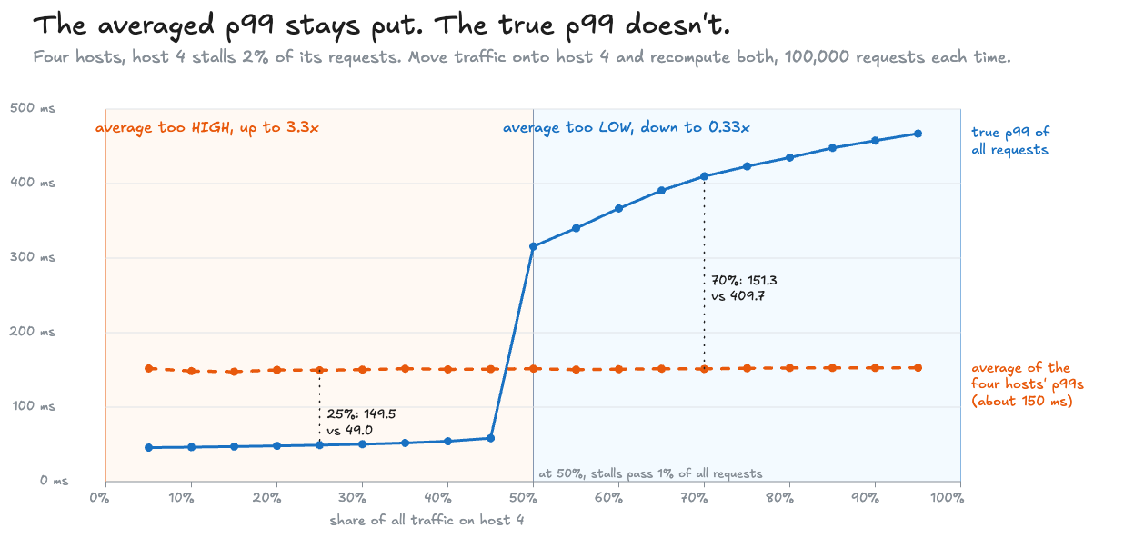
The averaged line is flat. It moves by about 5 ms across the whole range, while the true p99 moves by 421 ms.
Try it. The lab runs the same model in the page, with the same seed, so it starts at the post’s numbers. Drag Traffic on host 4 slowly to the right. At 50%, the solid line, the true p99, jumps over the dashed one, the average. Put it back at 25% and push Host 4 stalls past 4%, and the same jump happens, because 4% of a quarter of the traffic is 1%. Drag Calls per page to see the simulated pages track the formula. The Threshold slider belongs to the next section:
This lab runs a real call in your browser, so it needs JavaScript.
Add counts, then divide
There’s a version of “how slow is it” that rolls up exactly, and it’s the one head office uses. Instead of asking each host for a percentile, ask it for two counts: how many requests, and how many under 100 ms.
good = [sum(x < THRESHOLD_MS for x in h) for h in hosts]print(f"under {THRESHOLD_MS:.0f} ms: counts {good} sum to {sum(good):,} of {n:,} = {sum(good) / n:.3%}; " f"pooled {sum(x < THRESHOLD_MS for x in pooled) / n:.3%}")The first line counts, for each host, the requests strictly under the threshold. The second adds the four counts, divides by all 100,000, and prints that beside the share counted over every request at once:
...under 100 ms: counts [24896, 25196, 24954, 24471] sum to 99,517 of 100,000 = 99.517%; pooled 99.517%...The sum of four hosts’ counts is the count for the service, and the same goes for sixty minutes into an hour. It doesn’t matter how the traffic is split. In the 70% run the counts sum to 98.598%, and so does the pooled share. Averaging the four hosts’ percentages instead gives 99.499%. That’s the same mistake as averaging percentiles, in a smaller form, because a percentage needs its denominator just as a mean does. In the lab above, drag Threshold and the readout for requests under it shows the summed count, the count over all 100,000 at once, and the averaged shares, at every setting. Below 100 ms the share moves. Between 100 and 300 ms it can’t, because nothing takes that long except a stall.
This is how the Google SRE workbook defines a latency indicator: “the proportion of requests that are faster than defined thresholds” (Implementing SLOs). An SLO, a service level objective, adds a target and a window for that share: say, 99.5% of requests under 100 ms in every minute. That’s head office’s promise. A per-minute target and a monthly one are different promises, even when the percentage is the same.
Amazon CloudWatch makes both points concrete. It has the share as a statistic of its own, percentile rank: “PR(:300) returns the percentage of data points that have a value of 300 or less” (CloudWatch statistics definitions). And its SLOs make you pick between the two kinds of promise: a period-based SLO’s “attainment rate is calculated as the number of good periods/number of total periods,” while a request-based SLO “measures number of good requests/number of total requests during the interval” (Service level objectives).
That’s also why Prometheus, a widely used metrics system, has two ways to record latency that look alike and behave differently. A summary computes quantiles (another word for percentiles) on each instance. The documentation is blunt about what averaging them gives: “averaging the quantiles yields statistically nonsensical values” (Histograms and summaries).
A histogram records counts instead. The classic kind has a set of buckets, each with an upper edge, and each bucket counts every request at or under its edge. The edge is a label called le, short for less or equal, so the le="0.1" bucket counts every request that took 0.1 seconds or less. Counts add, so buckets from different instances add too. The same documentation page shows both queries:
avg(http_request_duration_seconds{quantile="0.95"}) // BAD!histogram_quantile(0.95, sum by (le) (rate(http_request_duration_seconds_bucket[5m]))) // GOOD.The first averages per-instance quantiles, which is the 149.5 ms mistake above, for a p95. The second adds the instances’ bucket counts over the last five minutes (rate(...[5m])), grouped by (le) so each bucket edge is summed separately, and then estimates one quantile from the total. That is the counterpart of the pooled 49.0 ms. It is an estimate, though, and only as fine as the bucket edges.
What a bucket does give exactly is the share of requests at or under its edge. So put a bucket edge at every threshold you promise. With an edge at 100 ms, the share at or under 100 ms is exact, summed across every instance and every minute. Keep the boundary straight, though: the demo counts requests under 100 ms, and a Prometheus bucket counts those at or under it. They differ only when a measurement lands exactly on the edge.
This tool does that rollup for your own histograms. It answers one question: what is the service’s real percentile across every instance, and how wrong is the averaged one?
Paste any of these, then press Run:
- each instance’s
_bucketlines, as a/metricspage or a query shows them; - a CSV of instance,
leand count; - raw latencies, one group per host, separated by a blank line;
- a cloud provider’s histogram: Google Cloud Monitoring’s JSON for a distribution metric, AWS X-Ray’s response-time histogram, or a CloudWatch Logs Insights or Azure KQL query that counts requests per duration bin. Amazon’s and Azure’s managed Prometheus return the Prometheus format. CloudWatch and Azure Monitor metrics keep only a percentile or an average per period, which can’t be pooled, so the tool refuses them and says where the counts are.
You get:
- the percentile estimated from the summed buckets, edge by edge, the way
histogram_quantiledoes; - how far off that estimate can be, which is the width of the bucket it lands in;
- the exact share under every bucket edge;
- the averaged per-instance percentile, for contrast.
The first two samples are the post’s two runs, all 100,000 requests counted into the Prometheus client’s default buckets (the companion code’s make_tool_samples.py), and they show the averaged p99 wrong in the same two directions as above:
| Sample | p99 from summed buckets | Somewhere between | Averaged per instance | True p99 |
|---|---|---|---|---|
| Equal split | about 50 ms | 25 and 50 ms | 149.2 ms | 49.0 ms |
| 70% of traffic on host 4 | about 370 ms | 250 and 500 ms | 152 ms | 409.7 ms |
The bucket edges are what keep the estimate from matching 49.0 and 409.7 exactly.
The wait your load test never timed
All of that assumes the measurements include the waits we care about. A load test, a program that sends requests at a server on a schedule and times the replies, can leave many of them out before any percentile is computed. In kitchen terms: a kitchen that times each order from when the cook picks up the ticket, rather than from when the customer ordered, never sees the queue of tickets on the rail.
A typical load-test loop sends a request, waits for the reply, records how long it took, and sends the next. Picture it against a server that freezes for 200 ms, with the client meant to send a request every 5 ms. The request in flight when the freeze starts waits about 200 ms, and it’s recorded as one slow request. During the freeze the client sends nothing, because it’s waiting. When the freeze ends it sends the 39 requests it owes, back to back. Each is answered in a fraction of a millisecond, and each is recorded as fast. A user who arrived during the freeze would have waited, but the test never sent that user’s request on time, so it never measured the wait.
Gil Tene named this coordinated omission. In the wrk2 README he describes it as “high latency responses result in the load generator coordinating with the server to avoid measurement during high latency periods.”
The fix is to time each request from when it was due on the schedule, rather than from when it was sent. The companion experiment does exactly that. It runs a real TCP server on a laptop, in a process of its own, and once a second the server freezes for 200 ms, then serves for the other 800 ms. Both runs use the same loop, and one line differs:
latencies.append((done - (due if from_schedule else sent)) * 1000)due is when the request should have gone out on the 5 ms schedule; sent is when it actually did. One 10-second run of each, 2,001 requests, times in milliseconds:
server freezes 200 ms every 1 s; client due to send 200 requests a second for 10 sfrom send time n= 2001 p50 0.18 p90 0.26 p99 1.02 max 205.25 mean 1.21 ms over 10 ms: 10from scheduled time n= 2001 p50 0.85 p90 106.45 p99 193.84 max 204.79 mean 21.91 ms over 10 ms: 392Timed from send, 10 requests took over 10 ms. Timed from the schedule, 392 did, and the p99 is 193.84 ms. The max is about 205 ms either way, because the ordinary loop does see each freeze, once. What it misses is how many requests each freeze affected.
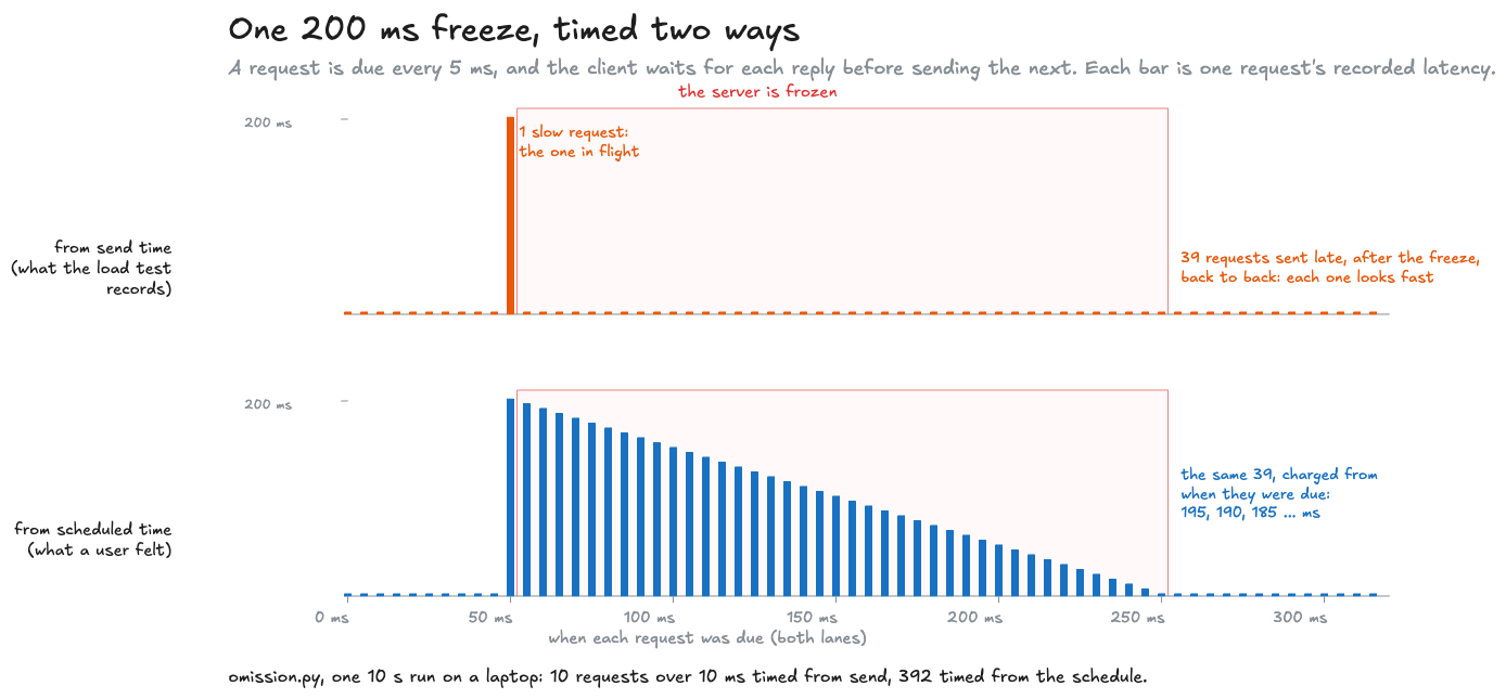
Timings depend on the machine, so here are seven runs on the same laptop. The scheduled-time p99 stayed between 192 and 196 ms. The counts over 10 ms stayed between 10 and 12 from send time, against 392 to 404 from the schedule. The send-time p99 is the number that wouldn’t sit still, anywhere from 0.7 to 5.7 ms, for the same reason host 4’s stalls hid from the p99 earlier. A freeze starts every second, so a 10-second run has ten of them, and each makes about one slow request timed from send. Ten or so out of 2,001 is under 1%, so the send-time p99 is just one of the dozen or so slowest ordinary round trips on the machine. A ratio built on it moves from tens to hundreds between runs, so I don’t quote one. The companion code’s CI checks the three stable numbers instead: the scheduled-time p99, and the two counts over 10 ms.
Why the server runs in its own process
The first version ran the server and the client in one Python event loop, and the freeze, a blocking time.sleep, froze the client too. The client then couldn’t even fall behind during the freeze, and the run measured the client’s own stall as much as the server’s. In a separate process only the server freezes, which is the situation a real load test is in. wrk2 corrects for coordinated omission the same way, timing from the intended schedule. The other fix is a load generator that sends on schedule without waiting for replies, which wrk2’s README notes only works for some protocols.
Either way, decide which workload the test models: users who arrive on their own schedule, or clients that really do wait for one answer before asking again. Only the first should be timed from the schedule.
What I’d put on the dashboard
Back to the checkout page. The service’s dashboard showed a mean and a p99, and neither one answered the customer’s question.
I’ve set latency targets as percentiles more than once: a p50 and a p90 for an ad system serving more than 100 requests a second, and a p99 for a real-time media framework with a 50 ms budget, where a change that made the p99 worse couldn’t merge. What I’ve learned to settle first, before the number itself, is which of the four questions a target answers and where it is measured. That decides how it’s stored and whether it can be added up.
For the checkout example, here’s what I’d keep, and what each number is for:
| Question | Number | How it rolls up | Alert on it? |
|---|---|---|---|
| How much capacity do we need? | Mean latency, with the request rate | Weighted by request count | No. Use it for sizing, with Little’s law, and keep headroom separate |
| How slow is a typical request, and a bad one? | p50 and p99, from a histogram | Only from summed bucket counts, never by averaging | Rarely: as a diagnostic beside the share |
| Did we keep the promise? | Share of requests under the threshold, over the SLO’s window, from histogram buckets | Exactly: sum the counts | Yes. This is the SLO |
| How slow are pages for people? | Page latency measured where the page is, or the share of slow pages | Counts again | Yes, for the team that owns the page |
| Is the measurement honest? | Load tests timed from the schedule | Not a dashboard number | Check once per load-test tool |
And for the team behind a call that a page fans out to 20 times: use the fan-out sum to agree their budget, then check it against real pages. For 20 independent calls, a 99% page target means 99.95% of calls under the threshold.
Run the model, then the measurement experiment
The code is in measuring-latency/, standard library only. latency_questions.py is the seeded model and every statistic above; omission.py is the real server and the two ways of timing it.
cd mainlog-code/measuring-latencypython3 latency_questions.py # the run quoted throughoutpython3 latency_questions.py --busy 0.7 # 70% of the traffic on host 4python3 latency_questions.py --csv sweep # the data behind the averaging chartpython3 omission.py # about 20 secondspython3 -m unittest discover -s testsThe model draws its random numbers with a small generator called mulberry32 rather than Python’s own, so the lab above, which runs the same code in JavaScript, draws the same 100,000 requests. Its CI checks every line of the model quoted here against a fresh run, and the coordinated-omission run against a band.
So when someone asks how fast the service is, the first thing I ask back is who wants to know: the manager, one customer, the table waiting for every dish, or head office.
Related posts
Code review economics
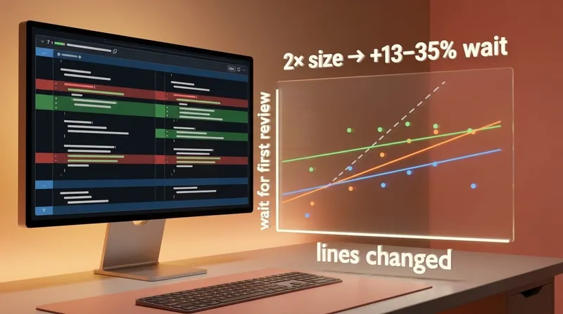
On three busy repositories the wait for a first review grows much more slowly than a PR's size, so a change split into eight PRs reviewed one after another waits three to eight times as long. Opening them side by side helps less than it looks, and only one reviewer taking them together is no worse than one PR. The measurement, the rule that falls out of it, and a tool to run it on your own PRs.
The unwritten rulescraftteamsstatistics
When to merge duplicate code
Whether two similar functions should become one depends on whether they change together, and git already knows. A real history from httpx, a script that counts co-changes across a repository, a browser tool for one pair, and a third answer that is neither copying nor abstracting: generate one copy and check it.
The unwritten rulescraftdesign-patternspython
Keeping optional Python imports optional
A test that checks importing a library leaves its optional dependency unloaded, and proves it got far enough to notice.
The unwritten rulespythontesting
 Software craft
Code review economics
On three busy repositories the wait for a first review grows much more slowly than a PR's size, so a change split into eight PRs reviewed one after another waits three to eight times as long. Opening them side by side helps less than it looks, and only one reviewer taking them together is no worse than one PR. The measurement, the rule that falls out of it, and a tool to run it on your own PRs.
craftteamsOct 2026 Software craft
When to merge duplicate code
Whether two similar functions should become one depends on whether they change together, and git already knows. A real history from httpx, a script that counts co-changes across a repository, a browser tool for one pair, and a third answer that is neither copying nor abstracting: generate one copy and check it.
craftdesign-patternsAug 2026 Software craft
Keeping optional Python imports optional
A test that checks importing a library leaves its optional dependency unloaded, and proves it got far enough to notice.
pythontestingAug 2026
Comments