More samples, same sound
Resampling makes a recording fit the next program. It can't restore what an earlier step filtered out.
Suppose you have a recording of a phone call and want to send it to a speech-to-text service. Before accepting it, the service asks you to convert the audio to a different sample rate.
Imagine it is a voicemail you want to turn into a searchable note. The useful result is a transcript of what the caller said. Getting the file accepted is one step toward that goal; it doesn’t yet tell you whether the words came through correctly.
That sounds like a routine format change. But what does the conversion actually do? Can it recover sound that the phone connection didn’t carry, or does it just make the existing recording readable by the next piece of software?
The distinction matters when you’re trying to improve an audio path. A recording can satisfy the receiving application’s format requirements while still missing part of the original sound. Increasing its sample rate won’t recover that missing part.
Let’s work out why, starting with what an audio file contains. Then we’ll use three simple beeps to watch a sound disappear during a conversion and check whether it comes back.
The short version
- A sample rate is how many measurements a second a recording keeps. Resampling recomputes them for a new rate and keeps the duration.
- A rate can only represent frequencies below half of it, so a proper conversion down to 8 kHz filters out everything above 4 kHz first.
- In the test with 1, 3 and 6 kHz tones, the 6 kHz tone was gone after 48 to 8 kHz, and stayed gone at 48 and at 16 kHz.
- Skipping the filter doesn’t keep it. The 6 kHz tone turned into a false 2 kHz one, and the file still passed a sample-count check.
opus/48000in a session description is the RTP timestamp clock. It says nothing about which frequencies survived.
From a beep to a list of numbers
Sound is a change in air pressure over time. A microphone turns that changing pressure into a changing electrical signal. To store it digitally, a recorder measures the signal at regular intervals and saves the measurements as numbers.
Each measurement is a sample. If the recorder takes 8,000 measurements in one second, its sample rate is 8,000 samples per second, usually written as 8 kHz. At 48 kHz, it takes 48,000 measurements per second. These counts are for one audio channel; stereo has a separate sequence for each channel.
The stored numbers describe the wave’s height at those instants. You’ll encounter this representation as PCM, or pulse-code modulation. MDN’s introduction to audio data explains how samples and channels make up a digital recording. The sample rate supplies the timing for those stored numbers.
Now think about the sound being measured. A pure tone is a simple, steady beep: one repeating, smoothly rising and falling wave. One complete repetition is a cycle. Its frequency tells us how many cycles happen each second. A 1,000 Hz tone repeats 1,000 times per second; a 3,000 Hz tone repeats three times as fast and has a higher pitch. “kHz” means thousands of hertz.
So we have two things to count. The sound wave repeats; the recorder takes measurements of it. Here is the same 1 kHz tone measured at two different rates:
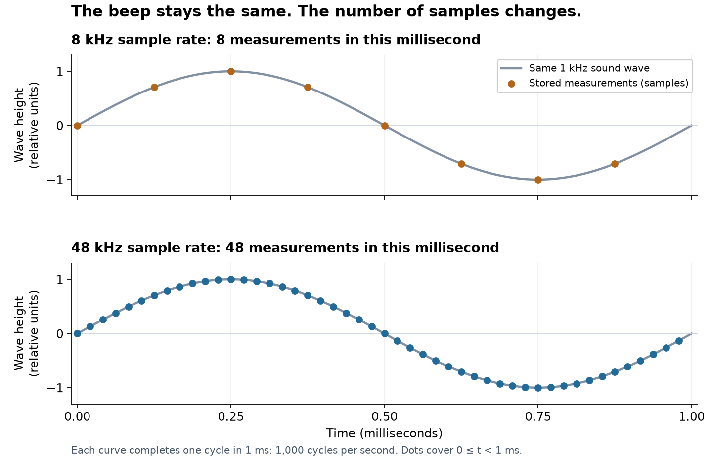
The smooth curve completes one cycle in both panels. At 8 kHz we store eight measurements of that cycle; at 48 kHz we store 48. The second panel hasn’t added a higher-pitched sound. It describes the same beep with more sample values.
A voice is more complicated than this single repeating wave. We can analyze it as a mixture of frequency components whose strengths change over time. When I talk about “missing detail” here, I mean components of the original sound that an earlier step removed. I don’t mean that the file contains too few bytes, or that a speech recognizer necessarily produced the wrong words.
Why the application asks for another rate
Back to the speech service. An audio endpoint defines the formats it accepts, including how many samples represent one second. That lets its processing code interpret the incoming numbers on the intended timescale.
For a concrete example, suppose our recording has 8,000 samples for each second, while the endpoint accepts 16,000. We need a new sequence containing 16,000 samples for that same second. Changing the label alone would make the receiver consume the original 8,000 samples in half a second, speeding up the recording and raising its pitch.
A resampler performs the actual conversion. It calculates a new set of sample values at the required spacing while preserving the recording’s duration. Producing more samples is called upsampling; producing fewer is downsampling.
That explains why we need the conversion even when it adds no sound detail. It makes the existing audio fit the receiver’s format and timing. The extra values are calculated from the information already available.
For a ten-second voicemail stored as single-channel PCM at 8 kHz, we have 80,000 samples. Converting it to 16 kHz produces 160,000 samples covering the same ten seconds. The caller should still speak at the same speed. That is a useful conversion: the service can now receive the representation it expects. The larger sample count is not evidence that we recovered more of the caller’s voice.
The question becomes more interesting when something was removed before those extra values were calculated.
Where a sound can get lost
A sample rate also limits which frequencies we can represent without ambiguity. If the measurements are too far apart, a rapidly changing wave can produce the same measured values as a slower one. The stored numbers alone cannot tell us which wave was there.
The Nyquist–Shannon sampling theorem gives the useful boundary: to represent a signal whose frequencies are below a particular limit, the sample rate must be more than twice that limit. Half the sample rate is commonly called the Nyquist limit. MDN’s digital audio guide introduces this relationship.
At 8,000 samples per second, that boundary is 4,000 Hz. A 1 kHz tone fits below it. So does a 3 kHz tone. A 6 kHz tone does not. Real filters need some room to transition between keeping and suppressing frequencies, so “below 4 kHz” is a theoretical boundary, not a promise that everything up to it survives unchanged.
Before reducing a recording to 8 kHz, a proper converter therefore suppresses the higher-frequency components that the new rate cannot represent correctly. The part doing that work is a low-pass filter: it keeps lower frequencies and reduces higher ones.
This is what a narrow frequency band means in this discussion: the recording retains a limited range of frequencies from the original sound. Audio bandwidth describes that range; it is a different quantity from the network bandwidth measured in bytes per second.
Once the high-frequency part has been suppressed, increasing the sample rate calculates more values from what remains. It doesn’t reveal what the original high-frequency part was.
I find that easier to see when we know exactly which sounds went into the recording.
Three beeps make the loss visible
We’ll generate three tones at once: 1, 3, and 6 kHz. Think of them as a lower, middle, and higher beep added together. Starting at a 48 kHz sample rate gives us room to represent all three.
Then we’ll reduce the rate to 8 kHz and return it to 48 kHz. If increasing the rate recovered the original sound, the 6 kHz tone would reappear. Finally, we’ll convert the result to 16 kHz for the illustrative endpoint from the opening.
This isolates the conversion itself. It isn’t a simulation of a complete telephone system, and we don’t need to guess which frequencies were present in somebody’s voice.
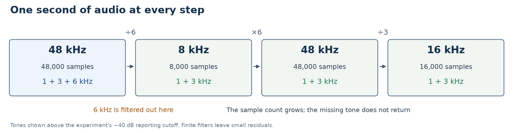
Every box represents the same one-second interval. The number of samples changes at each step, while the highest original tone falls out at the first downward conversion.
Here’s the result from the experiment:
| Stage | Samples representing one second | Original tones still prominent |
|---|---|---|
| Original at 48 kHz | 48,000 | 1, 3, and 6 kHz |
| Downsampled to 8 kHz | 8,000 | 1 and 3 kHz |
| Upsampled back to 48 kHz | 48,000 | 1 and 3 kHz |
| Converted to 16 kHz | 16,000 | 1 and 3 kHz |
The third row is the point. We are back to 48,000 samples, but the 6 kHz tone hasn’t returned. The final 16 kHz representation also has room for that tone (it could represent frequencies below 8 kHz), but the earlier step has already suppressed it.
The same issue can show up when editing a podcast. Suppose a guest interview arrived through a phone connection that removed some higher-frequency sound, and you export the episode at 48 kHz. The interview will be represented at the export rate, but that setting cannot recover what the connection removed. If the guest also made a local microphone recording, I’d compare that source before trying another conversion of the phone recording. The useful question is whether we have an earlier recording that still contains the sound we want.
We can inspect the sound rather than rely on the table. A frequency spectrum shows how strongly each frequency is present. A tall peak at 3 kHz means that the signal contains a strong component repeating 3,000 times per second.
In the figure below, the horizontal axis is frequency. The vertical axis compares each component’s amplitude with one of our original tones, using decibels (dB). Zero dB means the same amplitude as that reference. Negative values mean weaker components; −40 dB means one hundredth of the reference amplitude. It does not mean a sound is inaudible.
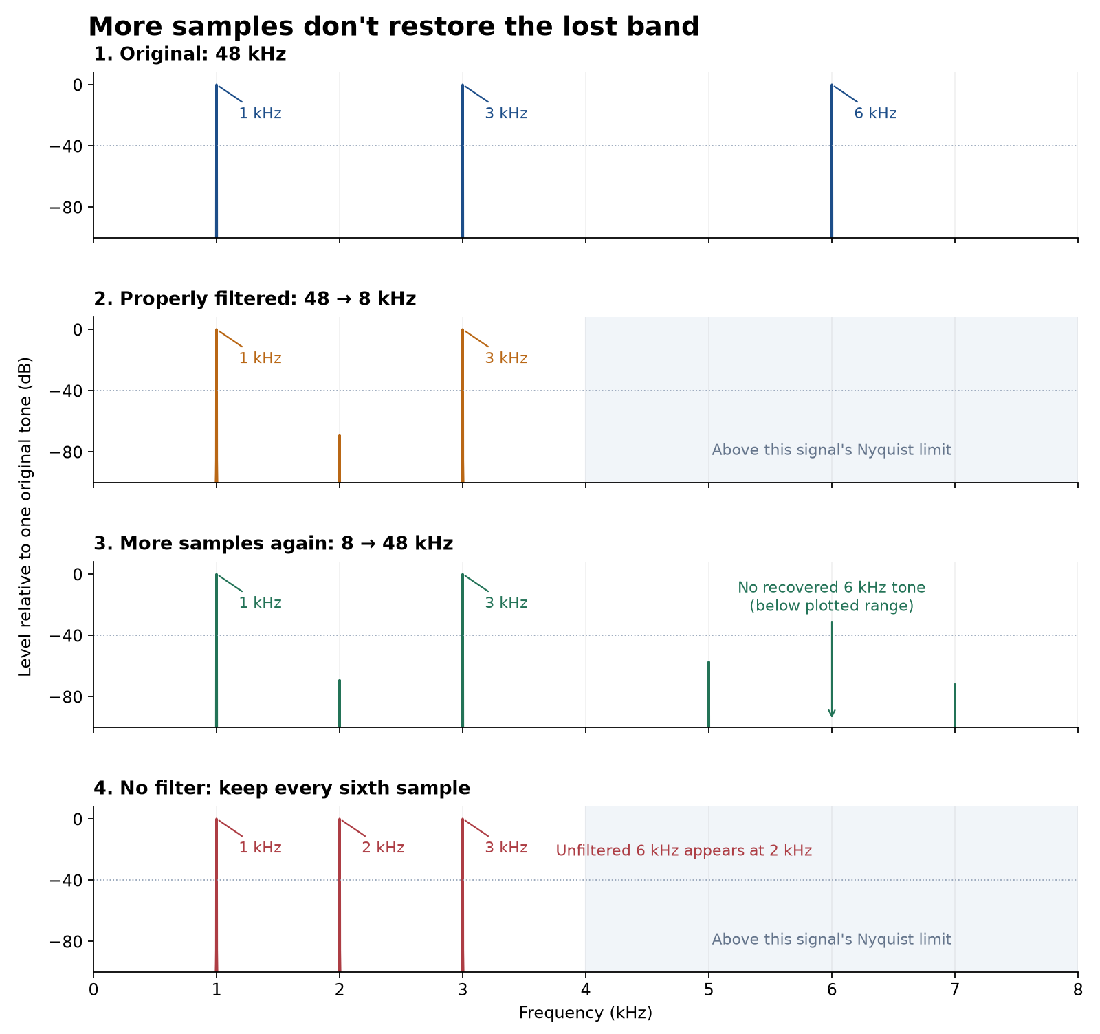
Read the first three panels in order: three strong peaks become two, and increasing the sample rate leaves them at two. The small peaks below the dotted reporting line are residuals and artifacts of finite filters; they aren’t a recovery of the original high tone.
The fourth panel answers a tempting question: could we keep the high tone by skipping the filter?
It takes every sixth sample from the original, giving the right count for 8 kHz. But now the 6 kHz tone appears as a false 2 kHz component. This is aliasing: one frequency becomes indistinguishable from another in the samples. For this particular input, the alias is |6000 − 8000| = 2000 Hz.
The conversion has introduced a sound at a frequency where our original had none. Filtering afterward cannot generally tell that false 2 kHz component apart from a genuine 2 kHz component. The high frequencies need to be suppressed before that ambiguity is introduced.
Try the conversion
The core experiment is small enough to run directly. NumPy creates the tones; SciPy performs the filtered conversions.
import numpy as npfrom scipy.signal import resample_poly
t = np.arange(48_000) / 48_000 # One second, sampled at 48 kHzoriginal = sum(0.25 * np.sin(2 * np.pi * f * t) for f in (1_000, 3_000, 6_000))
narrow = resample_poly(original, up=1, down=6)expanded = resample_poly(narrow, up=6, down=1)consumer = resample_poly(expanded, up=1, down=3)unfiltered = original[::6] # Deliberately wrong for this input
for name, samples, rate in [ ("original", original, 48_000), ("downsampled", narrow, 8_000), ("upsampled", expanded, 48_000), ("consumer", consumer, 16_000), ("unfiltered", unfiltered, 8_000),]: print(f"{name:12s} {len(samples):5d} samples " f"{len(samples) / rate:.3f} s")Each tone starts with an amplitude of 0.25. Adding them creates a single channel containing all three frequencies. The up and down arguments specify the rate ratio: 1 / 6 takes 48 kHz to 8 kHz, and 6 / 1 takes it back.
resample_poly includes the low-pass filtering. Its implementation organizes that filtering efficiently around the rate change, using a technique called polyphase filtering. We don’t need to implement a filter ourselves to reproduce the result.
Running the code produces:
original 48000 samples 1.000 sdownsampled 8000 samples 1.000 supsampled 48000 samples 1.000 sconsumer 16000 samples 1.000 sunfiltered 8000 samples 1.000 sNotice that even the deliberately wrong conversion passes a sample-count and duration check. Those checks establish timing; the spectrum reveals what happened to the sound.
The complete measurement script also checks the 1, 2, 3, and 6 kHz components. Its output is:
original 48000 Hz 48000 samples 1.000 s [1000, 3000, 6000]downsampled 8000 Hz 8000 samples 1.000 s [1000, 3000]upsampled 48000 Hz 48000 samples 1.000 s [1000, 3000]consumer 16000 Hz 16000 samples 1.000 s [1000, 3000]unfiltered 8000 Hz 8000 samples 1.000 s [1000, 2000, 3000]“Prominent” in the table means above −40 dB relative to one original tone. That is our reporting cutoff, not a hearing threshold, and a missing entry does not mean mathematically zero energy. The script measures the middle 0.8 seconds to avoid the edges of the finite recording, where the filter makes assumptions about the signal outside it.
The runs use Python 3.12.12, NumPy 2.5.3, and SciPy 1.18.1. The tested dependencies, short walkthrough, and figure generator are available together. After installing the dependencies, run python3 resampling_demo.py; python3 plot_experiment.py --out figures recreates the experiment figures. The introductory sound-and-samples figure has its own generator.
One more place that “48,000” can mislead
When debugging a networked voice application, there is another rate to keep separate. Opus is an audio codec: software that encodes audio into a compressed representation and decodes it back into samples. RTP, the Real-time Transport Protocol, carries media packets with timestamps that describe their timing.
For Opus over RTP, those timestamps use a 48,000-tick-per-second clock, regardless of the audio sampling rate or bandwidth. That’s specified in RFC 7587, section 4.1. Seeing opus/48000/2 in a session description therefore doesn’t establish that the recording retained high-frequency sound.
The decoder’s output sample rate is a separate choice. The Opus decoder API allows 8, 12, 16, 24, or 48 kHz. For 20 milliseconds of audio, the RTP clock advances by 48000 × 0.020 = 960 ticks. A decoder producing 16 kHz PCM outputs 16000 × 0.020 = 320 samples per channel for that same interval.
There is no timing disagreement: the two numbers count different units over the same duration. And neither says which sound frequencies survived earlier.
An 8 kHz stage is a real possibility in a voice path. For example, the PCMU and PCMA telephone audio formats have 8,000 Hz entries in RFC 3551’s payload table. That doesn’t describe every phone call, and a real telephone path can restrict the sound more than the theoretical 4 kHz sampling limit.
What I’d do with the recording
Back to our voicemail. I’d make the required conversion, check that the ten seconds still take ten seconds to play, and send it to the service. Then I’d judge the transcript against what the caller actually said. The service accepting 16 kHz audio establishes format compatibility; it doesn’t establish transcription accuracy.
If a word is wrong, I wouldn’t immediately blame the sample rate. I’d listen to the input and compare the transcript with a known reference. The tone experiment shows how frequency content can be lost; it doesn’t tell us how much that loss affects a particular speech recognizer. That needs a check with representative recordings.
For the podcast interview, the goal is different: retain the sound of the guest’s voice. If an earlier recording preserves detail the phone version lost, that’s the source I’d investigate. If the phone recording is all we have, repeated upsampling won’t reconstruct its missing original components.
Those examples lead to three practical checks:
- When the application rejects the format, convert correctly. Use its required sample rate and sample format. Verify the sample count against the duration so a label change doesn’t silently speed up playback.
- When required sound detail is missing, trace where it was lost. Compare a known input with the audio at successive boundaries. Address the narrowing capture or codec step, or use a better source recording where one exists. Keep the RTP timestamp clock separate from the PCM rate while inspecting the path.
- When the end result is disappointing, test that result directly. For transcription, check the words. For the controlled experiment, check the expected tones. A larger file or higher final sample rate is not the success criterion.
Resample to meet the next application’s format. Preserve the sound you need before it is lost. In our experiment, saving the 6 kHz tone means changing the 8 kHz step. In the voicemail workflow, success means the recording reaches the service at the right speed and the transcript is useful, not merely that the file now says 16 kHz.
Related posts
Observability-driven development
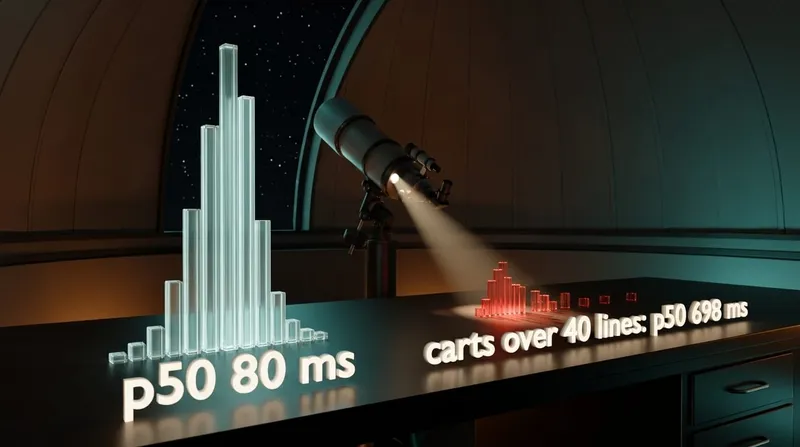
A deploy makes checkout slow for 0.9% of requests, and the dashboard's median doesn't move. Writing down the question you'd ask if it broke, and making a test prove the telemetry can answer it, is what finds them. Plus what that telemetry costs, in series and in microseconds.
Down to the wireobservabilitydistributed-systemstesting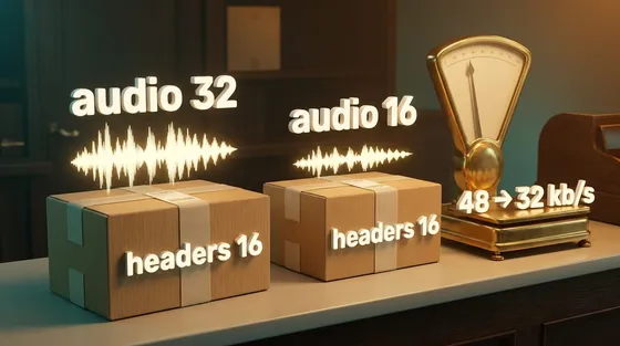
Half the bitrate, two thirds the traffic
Halving an audio bitrate from 32 to 16 kb/s took traffic from 48 to 32, because every packet's headers stay the same size. Packet rate is the other control.
Down to the wireaudionetworkingperformance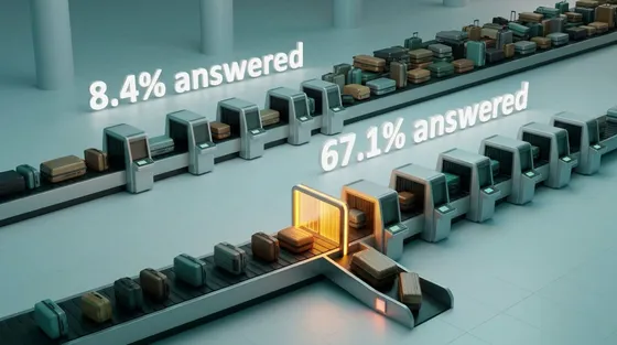
Backpressure and load shedding
A shop's checkout service can answer 100 requests a second, and for one minute 150 arrive. Left at the usual default, it answers 8% of those people in time; refusing the overflow at once answers two thirds. Capacity decides how many can be served. The policy decides whether they are, and only the question of who is a product decision.
Down to the wiredistributed-systemsreliabilityperformance
 Systems
Observability-driven development
A deploy makes checkout slow for 0.9% of requests, and the dashboard's median doesn't move. Writing down the question you'd ask if it broke, and making a test prove the telemetry can answer it, is what finds them. Plus what that telemetry costs, in series and in microseconds.
observabilitydistributed-systemsSep 2026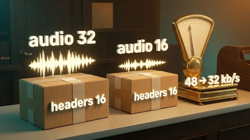 Networking & media
Half the bitrate, two thirds the traffic
Halving an audio bitrate from 32 to 16 kb/s took traffic from 48 to 32, because every packet's headers stay the same size. Packet rate is the other control.
audionetworkingAug 2026 Systems
Backpressure and load shedding
A shop's checkout service can answer 100 requests a second, and for one minute 150 arrive. Left at the usual default, it answers 8% of those people in time; refusing the overflow at once answers two thirds. Capacity decides how many can be served. The policy decides whether they are, and only the question of who is a product decision.
distributed-systemsreliabilitySep 2026
Comments